Gas flow measurement references

Definition and operating principle

Image

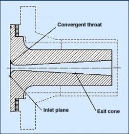
The critical flow Venturi nozzles (referred to below as sonic nozzles) used as transfer standards in France have a cylindrical throat whose geometry is defined in EN ISO standard 9300 [1]. 
Inserted into flow measurement systems, these nozzles have convergent and then divergent restrictions. The cylindrical convergent throat (inlet) is tangential to the inlet plane and to an exit cone through which the fluid escapes (figure 1).

The principle of sonic nozzles has been described by Saint-Venant, Stokes, Wilde and Reynolds. It is based on the fact that gas flowing through the nozzle accelerates to critical speed - equal to the speed of sound - at the throat. Using the principles of conservation of mass and isentropic expansion, we can show that mass flow through the nozzle at critical speed depends solely on conditions upstream of the nozzle. Critical speed is reached when the ratio between upstream and downstream pressure exceeds a certain level. The nozzle is then operating in sonic mode. Applying this theory, we can calculate mass flow through the nozzle (q_m) with the following formula:

$\displaystyle q_{m} = A_{*} \times f(y) \times\genfrac{}{}{1pt}{}{p_{0}}{\sqrt{(R/M)\times T_{0}}}$                               (1)

where f(y) is the critical flow function defined by:

$f(y)=\sqrt{y}\left (\genfrac{}{}{2px}{}{2}{y+1} \right )^{\genfrac{}{}{2px}{}{y+1}{2(y-1)}}$

and 

However, this formula is valid only if the following four conditions are met: 

• the gas is ideal ;
• the flow is isentropic ;                                                                                   (C1)
• the flow is one-dimensional ;
• the gas is static upstream of the nozzle.

In practice, the conditions (C1) are not verified. To determine mass flow from upstream conditions, formula (1) must be changed by introducing the critical flow function C_* and the discharge coefficient C_D, as follows:

$ \displaystyle q_{m} = A_{*} \times C_{D} \times C_{*} \times\genfrac{}{}{1pt}{}{p_{0}}{\sqrt{(R/M)\times T_{0}}}$                       (2)

Note: In practice, functions f(y) and C_* are equal only if the gas is ideal.

The critical flow function C_* used in formula (2) depends on the pressure (p₀) and stagnation temperature (T₀) of the gas upstream of the nozzle, and the nature of the gas. The critical flow function value for a number of gases can be calculated with an abacus. For example, the reference [1] gives critical flow values according to temperature and pressure for nitrogen, oxygen, argon, methane, carbon dioxide, air and water vapour. More sophisticated calculation methods are needed, however, to determine this function for more complex gases, such as natural gas (see AGA8-1992 and ISO 9300). The discharge coefficient used in formula (2) is the ratio between real flow and ideal flow if the conditions (C1) are met. In other words, this is a corrective coefficient that takes real conditions into account. By taking effects due to the gas into account in the critical flow function C_*, corrections for the gas are separated from corrections for the nozzle in the term C_D x C_*. In these conditions, a nozzle is calibrated by determining its discharge coefficient C_D experimentally, irrespective of the gas concerned.

In practice, formula (2) may also be used in an equivalent form (3) :

$ \displaystyle q_{m} = A_{*} \times C_{D} \times C_{R} \times \sqrt{ p_{0} \times \rho_{0}}$                           (3)

in which C_R is the critical flow coefficient for one-dimensional flow of a real gas equal to C_* x Z₀, with Z₀ the compressibility factor of the gas at the nozzle inlet.

Note: formula (3) can be demonstrated from formula (2) using the ideal gas equation.

When nozzles are calibrated, the discharge coefficient is determined for various values of the Reynolds number (Re_d) at the throat, using this formula (4):

$Re_{d} = \genfrac{}{}{1pt}{}{4 \times q_{m}}{\pi \times d \times \mu_{0}}$                                        (4)

where:

Advantages of sonic nozzles

Sonic nozzles are ideal instruments for measuring gas flow under pressure, for the following reasons:

• they have no moving parts and are hence highly stable
• mounting requirements are minimal
• their measurements are not affected by downstream flow conditions
• measurement uncertainties are low as they depend almost entirely on the accuracy of the measuring instruments
• each nozzle is calibrated by determining the value of its discharge coefficient (C_D,) as a function of the Reynolds number (Re), another adimensional quantity. The calibration curve is thus independent of the gas concerned.

The reliability of sonic nozzle technology is also confirmed by the results of comparisons [2].

The traceability chain set up by LNE-LADG comprises the PISCINE primary nozzle calibration bench and two secondary benches - HP M1 and PLAT - on which sonic nozzles are used as transfer standards (figure 2). These secondary benches use a comparison method for calibration of flow meters. They are located in Alfortville (Gaz de France) and Poitiers (CESAME).

Image

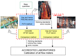
Figure 3 shows the traceability chain. It varies slightly according to the size of the reference sonic nozzle. If the nozzle throat is over 20 mm in diameter, an additional stage is necessary.

Image

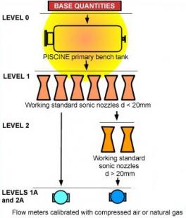
Level 0: LNE calibrates the volume of the PISCINE primary bench tank using a gravimetric method with water density as a traceability source. The sensors used to mesure density, pressure, temperature and voltage are calibrated by LNE. The chonometers are calibrated by the Observatoire de Besançon.

Level 1: Each sonic nozzle with a diameter under 20 mm is calibrated individually under pressure with the PISCINE primary bench, using the PVTt (pressure, volume, temperature and time) method. The discharge coefficient of each nozzle is determined for various Reynolds numbers by covering its entire operating range between 0.6 MPa and 5.5 MPa.

Level 2: Each sonic nozzle witha diameter over 20 mm is calibrated by comparison with a set of calibrated nozzles at level 1, using the LADG secondary benches. The discharge coefficient of each nozzle is also determined for various Reynolds numbers by covering its entire operating range.

Level 1A and 2A: External flow meters are calibrated by comparison with a set of sonic nozzles. The fluid used for calibration may be compressed air or natural gas.

Unlike laboratories in other countries, which calibrate nozzles on primary test benches using a mass method, LNE-LADG chose a volumetric calibration method. When its bench was designed in the early 1970s, existing technologies could not deliver acceptable measurement uncertainties with the mass method. The volumetric method (also called PVTt - pressure-volume-temperature-time) consists in determining the discharge coefficient C_D using a collection tank of known volume placed in series with the nozzle to be calibrated. Gas masses are determined from known volumes in the installation, and densities are determined by pressure and temperature measurements. The whole installation is immersed in a thermostatted water bath to maintain gas temperature at (20±2) °C during measurement. The operating principle is shown in figure 4 below.

Image

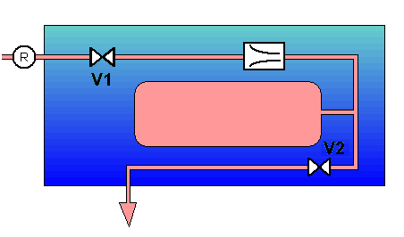
Stage 1: Valves V1 and V2 are open. Natural gas passes through the nozzle and is the evacuated to the bench's low-pressure outlet. Pressure regulator R sets pressure upstream of the nozzle to reach critical mode. Pressure downstream of the nozzle is close to the outlet pressure. After stabilization, initial conditions (density in the tank and the piping between V1 and V2) are determined.

Stage 2: Valve V1 stays open and V2 is closed. The gas passes through the nozzle and accumulates in the tank. Pressure downstream of the nozzle increases, but pressure regulator R maintains the ratio betwee, upstream and downstream pressure to maintain critical mode.

Stage 3: Valves V1 and V2 are closed. Pressure between V1 and V2 reaches equilibrium. After stabilization, final conditions (density in the tank and the piping between V1 and V2) are determined.

Following the procedure shown in figure 4, the gas mass between valves V1 and V2 in the initial state is calculated as follows:

$M_{initial} = \rho_{initial\_reservoir} \times V_{reservoir} + \rho_{final\_canalisations} \times V_{canalisations}$                           (5)

And in the final state:

$M_{final} = \rho_{initial\_reservoir} \times V_{reservoir} + \rho_{final\_canalisations} \times V_{canalisations}$                         (6)

Densities are calculated from pressure and temperature measurements and compressibility coefficients. Volumes are obtained by calibration.

Using formulas (5) and (6), mass flow through the nozzle during time t is calculated as follows:

$q_{m} = \genfrac{}{}{1pt}{}{M_{final} - M_{initial}}{t}$                             (7)

Using formulas (3) and (7), the discharge coefficient can be calculated:

$C_{D} = \genfrac{}{}{1pt}{}{q_{m}}{A_{*} \times C_{R} \times \sqrt{p_{0} \times \rho_{0}}}$                               (8)

Note: in practice, the product A_* x C_Dis determined directly during calibrations.

The creation of a reference value for natural gas flow measurement is the result of close cooperation between three European national metrology laboratories possessing references for high-pressure natural gas flow. PTB (Germany) and NMi-VSL (Netherlands) harmonized the value of their high-pressure natural gas cubic metre in June 1999, and LNE-LADG joined this harmonization agreement in May 2004. The principle of the agreement has been covered in several papers ([3], [4]). Under its terms, the participating laboratories must:

• possess an independent traceability chain
• demonstrate the stability of their references over a period of several years
• correct their measurements to obtain a reference value.

The corrections to be made are determined by comparisons.

The harmonized reference value (HRV) is based on a minimum of three independent references. It is calculated from the weighted average of the different reference values, using this formula:

$\displaystyle VRH = \sum_{i = 1}^{n}(W_{lab,i} \times V_{lab,i})$                                                  (9)

where v_lab,i is the value measured by laboratory i and w_lab,i is the weighting for this laboratory's measurement, defined thus:

$\displaystyle W_{lab,i} = \genfrac{}{}{1pt}{}{1}{1 + U_i^2 \times \sum \limits_{\underset{k \neq i}{k=1}}^n (1/U_K^2)}$             (10)

with U_k the increased uncertainty of laboratory k.

Note: this formula ensures higher weighting for a low-uncertainty measurement.

With these notations, the increased uncertainty on the value of HRV is:

$\displaystyle U_{VRH} = \sqrt{\sum_{i=1}^{n}(W_{lab,i}^2 \times U_{lab,i}^2)}$                       (11)

PISCINE primary bench

The product (A_* x C_D) can be measured directly with the PISCINE primary bench.

PLAT secondary bench

On the PLAT secondary bench the meter is mounted in series with one or more standard sonic nozzles.
With calibration we determine:

• the variance between the standard flow and the flow measured by the meter during tests
• or the discharge coefficient if negative pressure devices or sonic orifices are calibrated.

M1 secondary bench

On the M1 secondary bench the meter is mounted in series with one or more standard sonic nozzles. 
With calibration we determine:

• the variance between the standard flow and the flow measured by the flow meter or meter during tests
• or the discharge coefficient if negative pressure devices or sonic orifices are calibrated.

[1] :   AFNOR, « Mesure de débit de gaz au moyen de Venturi-tuyères en régime critique », NF EN ISO 9300, August 2005.

[2] :   MICKAN B., KRAMER R., DOPHEIDE D., HOTZE H-J, HEINO-MICHAEL HINZE, JOHNSON A., WRIGHT J. et VALLET J.-P., “Comparisons by PTB, NIST, and LNE-LADG in air and natural gas with critical Venturi nozzles agree within 0.05 %”, 6th ISFFM, Queretaro, Mexique, 16-18 May 2006.

[3] :   VAN DER BEEK M.J., LANDHEER I.J., MICKAN B., KRAMER R. et DOPHEIDE D., "Unit of volume for Natural gases at operational conditions: PTB and NMi-VSL disseminate Harmonized Reference Values", Proceedings of 2003 FLOMEKO Conference, Groningen, Netherlands, May 2003.

[4] :   MICKAN B., KRAMER R., DOPHEIDE D., VAN DER BEEK M.J. ET BLOM G.., “The harmonized high-pressure natural gas cubic meter in Europe and its benefit for user and metrology”, Proceedings of 2004 FLOMEKO Conference, Guilin, China, September 2004.